If you have any questions about the code here, feel free to reach out to me on Twitter or on Reddit.
Shameless Plug Section
If you like Fantasy Football and have an interest in learning how to code, check out our Ultimate Guide on Learning Python with Fantasy Football Online Course. Here is a link to purchase for 15% off. The course includes 15 chapters of material, 14 hours of video, hundreds of data sets, lifetime updates, and a Slack channel invite to join the Fantasy Football with Python community.
Correlation coefficients
In this part of the machine learning/statistics series, we are going to examine our model further using correlation analysis. We'll be circling back to our root mean squared error of 26 and what that number means to us in the next post.
If you have not yet checked out part one of the series, here's the link to that.
We'll be doing this using the correlation coefficient, which measures the extent to which the relationship between two variables is linear. It's value is a function of covariance normalized to somewhere between -1 and 1 (covariance isn't all that useful to look at on it's own, which is why it's value is normalized and why we use correlation instead). 1 means two variables are perfectly positively correlated (when one variable goes up 10%, the other goes up 10%), and -1 means two variables are perfectly negatively correlated. 0 means there is absolutely no correlation. Before we jump in to analyzing Fantasy Football, let's run some examples using numpy and random numbers.
What we did here is we defined some sample data x, which is just a bunch of random numbers generated for us by numpy. This function randn draws from a uniform distribution over [0, 1] - meaning, all of our random sample values are somewhere between 0 and 1.
We then set a variable y equal to 2 times x, plus some random noise. The function normal randomly draws from a normal distribution.
We use the numpy function corrcoef to find the correlation matrix of the two variables. We get back a matrix here, but the value we want to look at is that .95. That's our correlation coefficient. That's a strong correlation, as was expected, considering we added only a bit of random noise.
We can increase the amount of random noise in our y by increasing the width of the distribution our normal function draws from. We do this by bumping the second argument of our np.random.normal function.
You can see now that our model has a correlation closer to 0 than before. In other words, it has become less correlated. This makes sense as we added in more random noise, decreasing the relative proportion of our model that was correlated to x (The 2*x part).
Here's how we would plot our two models. Below is what seaborn gets us back.
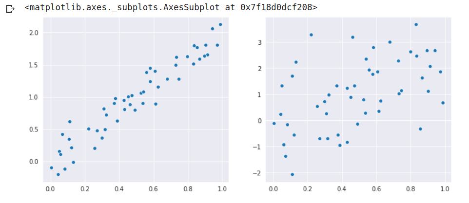
You can see that both kind of look correlated, but with the added noise the points in the second visualization are less tightly bunched together. This ties in to what we learned last time, the more tightly bunched together our data is around our model (the lower the summed squared residuals), the more predictive our model is. You can see that everything is starting to tie in to each other. The model we created in part one - you can can think of it as an optimization function, where the model is trying to create the line that optimizes the summed squared residuals to the lowest possible value. In other words, the line (or model) that minimizes the sum of the squared residuals. The better our model can optimize this summed squared residual value given our data, the better the correlation coefficient (closer to 1) and the more predictive our model.
Turning Back to Our Model
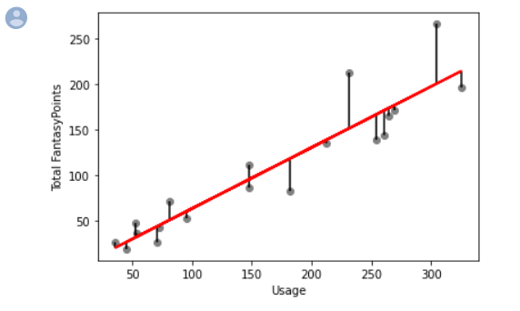
Now, given all this information, let's turn back to our model we created in part one. What is the correlation coefficient of the two variables we're examining - usage and Fantasy Football performance? This won't require a ton of code, actually.
By the way, "correlation coefficient", "coefficient of determination", and "R squared" are all used to denote the same thing. You can see that our correlation of coefficient of determination for our model is 0.86. That's quite good.
We'll be working on this model again in the next post, next time writing a bit more code. Thanks for reading, you guys are awesome!