If you have any questions about the code here, feel free to reach out to me on Twitter or on Reddit.
Here's a link to the CSV file we'll be using throughout this post.
Shameless Plug Section
If you like Fantasy Football and have an interest in learning how to code, check out our Ultimate Guide on Learning Python with Fantasy Football Online Course. Here is a link to purchase for 15% off. The course includes 15 chapters of material, 14 hours of video, hundreds of data sets, lifetime updates, and a Slack channel invite to join the Fantasy Football with Python community.
Welcome Back, Some Updates, and Introductions
Just a few updates: The course I've been working on to Learn Python for Fantasy Football is out now! If you're interested in learning Python from scratch definitely give it a try.
In this post, we're going to begin a string of posts on Machine Learning. I think something like this is probably going to necessitate a series on it's own.
Finally, big thanks to Frank Bruni for providing the source code for this series! We'll be working together in this series on co-writing posts.
Enough introductions. Let's talk about what machine learning is and how we'll be using it.
What's Machine Learning?
Most of you have probably heard the word Machine Learning before. It's a buzzword and sounds kinda scary, and the math behind the algorithms can get quite complicated. But the implementation of these algorithms in Python using a library known as sklearn is actually quite straightforward.
Typically, a computer program is a series of instructions you explicitly define for the computer/server/whatever to run, and it just does it - assuming you told it correctly how to do what it needs to do (you used proper syntax).
ML, on the other hand, is great because ML algorithms allow a computer to complete tasks based off past data without us having to explicitly define how to make those predictions. It does this by learning or "training" with previous data.
Moreover, machine learning algorithms typically fall in to two camps - either supervised or unsupervised. Supervised ML algorithms learn on labeled data, while unsupervised algorithms do not need labels (and are typically used to come up with labels for supervised algorithms). Learning with labels means that when the algorithm learns, it takes in some feature matrix usually denoted as X, and also takes in some target array, usually denoted by y, and then tries to come with a way of describing the relationship between the feature matrix and the target array. This function that the algorithm comes up with is what the algorithm is trying to learn. Then, we can take data that has no labels and use our new function to predict a new label for our unseen data.
Supervised and unsupervised machine learning algorithms can be broken down even further.
Unsupervised algorithms can be broken down in to clustering algorithms, and dimensionality reduction algorithms. Clustering algorithms aim to find distinct groups within a data set. Dimensionality reduction algorithms aim to find some lower dimensional representation of a large data set, while keeping many of the essentialities of the original data set (essentially finding a more succinct representation).
For supervised algorithms, we have regression and classification algorithms. Regression algorithms predict a continuous value - a value that can span any interval, for example, fantasy football points. Classification algorithms aim to predict which class an input belongs to. There are many regression algorithms and classification algorithms that we won't be able to cover. We are going to start with the simplest, Simple Linear Regression, then move on to Multiple Linear Regression, and then add regularization to our model with cross-validation.
Applying it to Fantasy Football
If you've been following my previous intermediate series, you know that in part one of the series, we examined running back usage (Basically, number of carries and number of targets) and found the correlation to fantasy points scored per game. We found that the two variables were pretty highly correlated. (We also examined running back efficiency versus fantasy points scored per game and found that efficiency was not as nearly highly correlated. Takeaway: prioritize usage over efficiency when choosing running backs).
But what if we could use that insight to make actual predictions on fantasy football performance?
What if we could take previous years running back stats to train a model and make predictions on running back FF performance for future years (like 2020)? (If you've been following along my other posts, you'll know that we have access to fantasy data all the way back to 1999. That's part four of the intermediate series on web scraping. We can use all this data to train our model. I've recently made this data freely available for download straight off the FFDP site. Navigate to ).
How We'll Be Using ML in this Part
What we'll be doing in this post is creating a regression model to predict Fantasy Football performance based solely off our 2019.csv we've used previously. The way we do this is by using some portion of our dataset to train our model and then use the rest to see how well the model performs.
We'll be splitting the 2019 dataset up into 80% train and 20% test. Meaning we'll be using 80% of the dataset to train our model, and test our model with the remaining 20%.
In future posts, we'll be increasing the amount of data we use to train the model.
Our First Block of Code
Just importing some stuff. There's one new line of code and some other new libraries we're now importing that I want to point out but that's it.
This is the one new line that we haven't covered in previous posts, and basically all we're doing is suppressing a warning from pandas. Not a big deal and totally optional.
We're also importing two new methods/classes from sklearn which comes with our notebook environment (whether you're using colab or jupyter)
sklearn is shorthand for scikit-learn, and is probably the most popular Machine Learning library for Python. It is based on the Estimator API, which is very straightforward and allows us to use the same process for training and testing each algorithm in sklearn's arsenal.
That's pretty much it for this code block.
Our Second and Third Block of Code - Same Old
Read our csv file and import it. Clean up some row values with .apply(). Rename columns. Separate based off position. Considering you already read the first post of our intermediate series - you got this.
This is third cell is all stuff we've done before as well. Again, you all should be good on this stuff assuming you've gone through the intermediate series.
Briefly, though - we create a process to partition each of our DataFrames with the appropriate columns, which we define in rushing_columns, receiving_columns, and passing_columns. We then use a function we wrote called transform_columns to do this. Note we only do this for rb_df here because we are focusing on running back usage in this post, but you could have used transform_columns for other positions as well (just pass in the right arguments to transform_columns).
Next, we create the FantasyPoints and Total Usage columns and use .apply() to format and round some numbers. Easy enough.
Our First Lines of Machine Learning Code
Okay, so we're going to be looking at running backs for the rest of this post, much like we did in previous posts. You're welcome to do a similar analysis with other positions but I think it is interesting to look at running back usage since it is comprised of both rushing and receiving.
First step is we need to specify what data we want to predict. We want to use usage to predict fantasy points. So we'll use fantasy points as our dependent variable y since it depends on usage.
Let's run through this code step by step.
First, we set our x (independent variable) and our y variables equal to Usageand FantasyPoints, respectively. Remember, FantasyPoints depends on Usage.
Before we completely assign those variables, though, we have to reshape our columns.
Our function that we are passing our x and y values to requires that - first off, x and y be of the same dimensions.
So we use the .values attribute of our two columns to return a Numpy array representation of our DataFrame columns, and then use the .reshape(-1, 1) Numpy array method to reshape our two arrays into a single column, resulting with each now having a shape of (92, 1)
sklearn has a function that we imported earlier called train_test_split. Per scikit-learn documentation, train_test_split "splits arrays or matrices into random train and test subsets". We pass in three things to this function that scikit-learn gives us - Our X column, our y column, and the test size (what percentage portion of the population we want to use for testing).
You should understand by now why we're passing our x and y columns to train_test_split
test_size is, again, the percentage of our population we want to use for testing. By providing a value of 0.2, we are also saying that 80% of our population is going to be used for training our model.
Next, we create an instance of our Regressor class we imported from scikit-learn earlier.
We then pass in our training values we got from train_test_split into our regressor instance using the fit built in method.
Why do we pass in our training values? Because we need to create a model based off training values, and then test our model with the testing values - it's as simple as that.
So we "train" the model, and then we use it to predict FantasyPoints, our y column, with our x testing values. To reiterate one more time - we used our x and y training values to create or train our model - and now we are using that model we trained to predict FantasyPoints using our x testing values.
We now create a new DataFrame with our y_test and y_pred to compare our results. It's important to note that our y_test is our unaltered test values. They are actual Fantasy Points per game values we got from manipulating and transforming our original CSV file. Our y_pred values are the values we got from our model. So now, we are comparing actual, real world results to our model and seeing how we did.
Also, we use the .flatten() to collapse our arrays into a single column so that they can be passed in to our DataFrame.
We can look at each player and see how close we got to their actual fantasy point output and you can see we get pretty close. Check out the results and see how we did.
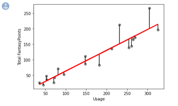
Finally, our last bit of code to produce our visualization. This post is getting kinda long so I want you to make what you will of the visualization for now. We'll be covering it in more detail part two. In part two, we're going to explain in detail more about this visualization - what it means, and how we can make it better and what "better" means. For now, treat this as an exercise and study the visualization and try to make sense of it. The code is pretty self explanatory even though we haven't covered making visualizations this way (we've been using seaborn mostly), but we'll be covering that too.

Conclusions
Thanks for reading guys, hopefully this post showed you that machine learning isn't that scary and you learned something from it. Over the next couple weeks, assuming we're all still in quarantine - I'll be posting a lot more free content to keep you guys productive :)
Special thanks again to Frank Bruni for making this post happen!