If you have any questions about the code here, feel free to reach out to me on Twitter or on Reddit.
Shameless Plug Section
If you like Fantasy Football and have an interest in learning how to code, check out our Ultimate Guide on Learning Python with Fantasy Football Online Course. Here is a link to purchase for 15% off. The course includes 15 chapters of material, 14 hours of video, hundreds of data sets, lifetime updates, and a Slack channel invite to join the Fantasy Football with Python community.
What We'll Be Doing in This Part
If you haven't read part one of the Machine Learning series, check it out here.
In this part of the machine learning series, we'll be building up on our past model and introducing a few new concepts. We won't be writing a ton of code in this part, but we will be introducing a ton of new statistical concepts to help you think about our models.
Standard Deviation
To start, let's talk about standard deviation. Some of you may already know what standard deviation is, or at least have a general idea of what it may be, but do not know exactly what it means. Standard deviation is simply a number representing how dispersed our data set is. It's a numeric measure of how spread out our data is. Is our data closely bunched together around the average (mean), or is it spread out?
Standard deviation is a function of variance. Simply put, the standard deviation of a data set is the square root of it's variance.
There are other measures of dispersion as well, such as mean absolute deviation, which measures the average of the absolute deviations away from the mean. Standard deviation is more widely used than MAD because it is mathematically easier to deal with. Similarly, we more commonly use standard deviation over variance when describing data because standard deviation is conveniently in the same units as our data.
For example, let's say we have a data set of running back season projections. We can have a mean of let's say 150 Fantasy Points (this is hypothetical) and have a standard deviation of 20 Fantasy Points. This basically means that a lot of our running back stats lies in a +-20 range of our mean, or in the 130 to 170 range. If instead, we had a standard deviation of 40, this would mean that a lot of our data lies in that 110 to 190 range - a much larger range. I'm simplifying things here, but you get my point.
In my course on learning Python with Fantasy Football, we actually examine these numbers for each position - and we find that actually running back projections are the most dispersed (have the most standard deviation).
Root Mean Square Deviation
That heading is scary, but it's actually not and it's the topic of this post. It ties in to what we've been talking about with standard deviation.
In the last post, we used usage to predict Fantasy Points. We want to figure out a way to quantify how our model did.
One way to do this is to calculate the standard deviation of the residuals. When I say residual, I mean the difference between our model's predicted Fantasy Points and actual values, or in the simplest terms possible, our models error.

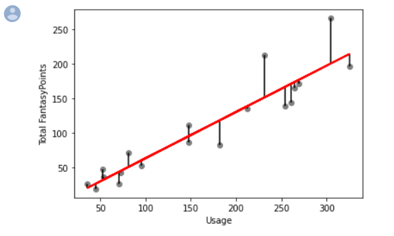
Remember last time we created this visualization to show how our model did. Essentially, the red line is our model. The scatter points is what happened in real life. The closer or less dispersed these scatter points are around our model or line of best fit, the better predictive value our model had.
The way to describe this dispersion around the line of best fit we generated here is to calculate what's called the Root Mean Squared Deviation. This statistic is the quantified measure of how dispersed our residuals are around that line of best fit.
Let's take a look at our previous model, this time with a visual representation of our "residual" plotted as well. We can easily do this using a method that comes with matplotlib called vlines. We call this method right off our ax object we create using fig, ax. Let's go back to our model from part one and alter the code a bit.
And below is what matplotlib gives back to us. You can see below that the black lines represent the vertical distance of each data point to our model. This is our residual. What we want to do is take these vertical distances, square them, sum them all up, and then take the square root of the sum.
Thankfully, scikit makes this extremely easy for us, so this part won't contain a lot of code.
In the same notebook as we used last time, input this into the cell below.
We get back around 26 as our result. This is the standard deviation of our residuals, meaning most of our predictions we made with our model are within 26 Fantasy Points. Is this good enough? That's for you to decide and for us to examine in part 2 of the Machine Learning / stats series. Thanks for reading :)